keras 人工智能之VGGNet神经网络模型训练
上期文章我们分享了如何使用LetNet体系结构来搭建一个图片识别的神经网络:
人工智能Keras的第一个图像分类器(CNN卷积神经网络的图片识别)
本期我们基于VGGNet神经网络来进行图片的识别,且增加图片的识别种类,当然你也可以增加更多的种类,本期代码跟往期代码有很大的相识处,可以参考
VGGNet基础
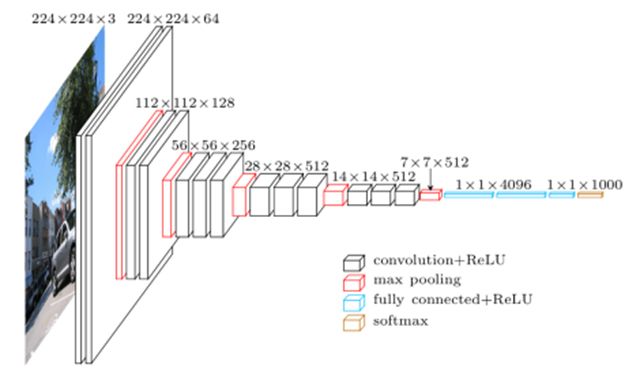
VGG16结构图
- 输入是大小为224*224的RGB图像,预处理(preprocession)时计算出三个通道的平均值,在每个像素上减去平均值
- 图像经过一系列卷积层处理,在卷积层中使用了非常小的3*3卷积核,在有些卷积层里则使用了1*1的卷积核。
- 卷积层步长(stride)设置为1个像素,3*3卷积层的填充(padding)设置为1个像素。池化层采用max pooling,共有5层,在一部分卷积层后,max-pooling的窗口是2*2,步长设置为2。
- 卷积层之后是三个全连接层(fully-connected layers,FC)。前两个全连接层均有4096个通道,第三个全连接层有1000个通道,用来分类。所有网络的全连接层配置相同。
- 全连接层后是Softmax,用来分类。
- 所有隐藏层(每个conv层中间)都使用ReLU作为激活函数。VGGNet不使用局部响应标准化(LRN),这种标准化并不能在ILSVRC数据集上提升性能,却导致更多的内存消耗和计算时间(LRN:Local Response Normalization,局部响应归一化,用于增强网络的泛化能力)。
VGGNet keras 神经网络搭建
使用VGGNet基础知识,我们使用keras来搭建一个小型的神经网络,新建一个smallervggnet.py文件
from keras.models import Sequential
from keras.layers.normalization import BatchNormalization
from keras.layers.convolutional import Conv2D
from keras.layers.convolutional import MaxPooling2D
from keras.layers.core import Activation
from keras.layers.core import Flatten
from keras.layers.core import Dropout
from keras.layers.core import Dense
from keras import backend as K
class SmallerVGGNet:
	@staticmethod
	def build(width, height, depth, classes):
		# initialize the model along with the input shape to be
		# "channels last" and the channels dimension itself
		model = Sequential()
		inputShape = (height, width, depth)
		chanDim = -1
		# if we are using "channels first", update the input shape
		# and channels dimension
		if K.image_data_format() == "channels_first":
			inputShape = (depth, height, width)
			chanDim = 1
		# CONV => RELU => POOL
		model.add(Conv2D(32, (3, 3), padding="same",
			input_shape=inputShape))
		model.add(Activation("relu"))
		model.add(BatchNormalization(axis=chanDim))
		model.add(MaxPooling2D(pool_size=(3, 3)))
		model.add(Dropout(0.25))
		# (CONV => RELU) * 2 => POOL
		model.add(Conv2D(64, (3, 3), padding="same"))
		model.add(Activation("relu"))
		model.add(BatchNormalization(axis=chanDim))
		model.add(Conv2D(64, (3, 3), padding="same"))
		model.add(Activation("relu"))
		model.add(BatchNormalization(axis=chanDim))
		model.add(MaxPooling2D(pool_size=(2, 2)))
		model.add(Dropout(0.25))
		# (CONV => RELU) * 2 => POOL
		model.add(Conv2D(128, (3, 3), padding="same"))
		model.add(Activation("relu"))
		model.add(BatchNormalization(axis=chanDim))
		model.add(Conv2D(128, (3, 3), padding="same"))
		model.add(Activation("relu"))
		model.add(BatchNormalization(axis=chanDim))
		model.add(MaxPooling2D(pool_size=(2, 2)))
		model.add(Dropout(0.25))
		# first (and only) set of FC => RELU layers
		model.add(Flatten())
		model.add(Dense(1024))
		model.add(Activation("relu"))
		model.add(BatchNormalization())
		model.add(Dropout(0.5))
		# softmax classifier
		model.add(Dense(classes))
		model.add(Activation("softmax"))
		# return the constructed network architecture
		return model
搭建图片识别训练模型
导入第三方库
import matplotlib
matplotlib.use("Agg")
from keras.preprocessing.image import ImageDataGenerator
from keras.optimizers import Adam
from keras.preprocessing.image import img_to_array
from sklearn.preprocessing import LabelBinarizer
from sklearn.model_selection import train_test_split
from smallervggnet import SmallerVGGNet
from keras.utils import to_categorical
import matplotlib.pyplot as plt
from imutils import paths
import numpy as np
import random
import pickle
import cv2
import os
初始化数据
EPOCHS = 100  #学习的步数
INIT_LR = 1e-3 #学习效率
BS = 32# 每步学习个数
IMAGE_DIMS = (96, 96, 3) # 图片尺寸
data = [] # 保存图片数据
labels = [] # 保存图片label
# 加载所有图片
imagePaths = sorted(list(paths.list_images("dataset\\")))
random.seed(42)
random.shuffle(imagePaths)
遍历图片搜集图片信息
for imagePath in imagePaths:
    # 加载所有图片
    image = cv2.imread(imagePath)
    image = cv2.resize(image, (IMAGE_DIMS[1], IMAGE_DIMS[0]))
    image = img_to_array(image)
    data.append(image)
		# 搜集图片data 与label
    label = imagePath.split(os.path.sep)[-2]
    print(label)
    labels.append(label)
处理图片
# 处理数据到0-1
data = np.array(data, dtype="float") / 255.0
labels = np.array(labels
# 标签二值化
lb = LabelBinarizer()
labels = lb.fit_transform(labels)
#labels = to_categorical(labels) #多类删除这个,当然本期代码完全可以使用在介绍lenet网络上
搭建神经网络模型
(trainX, testX, trainY, testY) = train_test_split(data,
                                                  labels, test_size=0.2, random_state=42)
#分开测试数据
#创建一个图像生成器对象,该对象在图像数据集上执行随机旋转,平移,翻转,修剪和剪切。
#这使我们可以使用较小的数据集,但仍然可以获得较高的结果
aug = ImageDataGenerator(rotation_range=25, width_shift_range=0.1,
                         height_shift_range=0.1, shear_range=0.2, zoom_range=0.2,
                         horizontal_flip=True, fill_mode="nearest")
# 初始化模型
model = SmallerVGGNet.build(width=IMAGE_DIMS[1], height=IMAGE_DIMS[0],
                            depth=IMAGE_DIMS[2], classes=len(lb.classes_))
opt = Adam(lr=INIT_LR, decay=INIT_LR / EPOCHS)
model.compile(loss="categorical_crossentropy", optimizer=opt,
              metrics=["accuracy"])
训练神经网络
H = model.fit_generator(
    aug.flow(trainX, trainY, batch_size=BS),
    validation_data=(testX, testY),
    steps_per_epoch=len(trainX) // BS,
    epochs=EPOCHS, verbose=1)
保存训练模型
model.save("VGGNet.model")
f = open("labelbin.pickle", "wb")
f.write(pickle.dumps(lb))
f.close()
显示训练结果
训练结果
plt.style.use("ggplot")
plt.figure()
N = EPOCHS
plt.plot(np.arange(0, N), H.history["loss"], label="train_loss")
plt.plot(np.arange(0, N), H.history["val_loss"], label="val_loss")
plt.plot(np.arange(0, N), H.history["acc"], label="train_acc")
plt.plot(np.arange(0, N), H.history["val_acc"], label="val_acc")
plt.title("Training Loss and Accuracy")
plt.xlabel("Epoch #")
plt.ylabel("Loss/Accuracy")
plt.legend(loc="upper left")
plt.savefig("plot1.JPG")
识别图片
下期我们将使用预训练好的模型对图片进行识别